The processes involved in this project are shown as a workflow diagram in Figure 1 below:
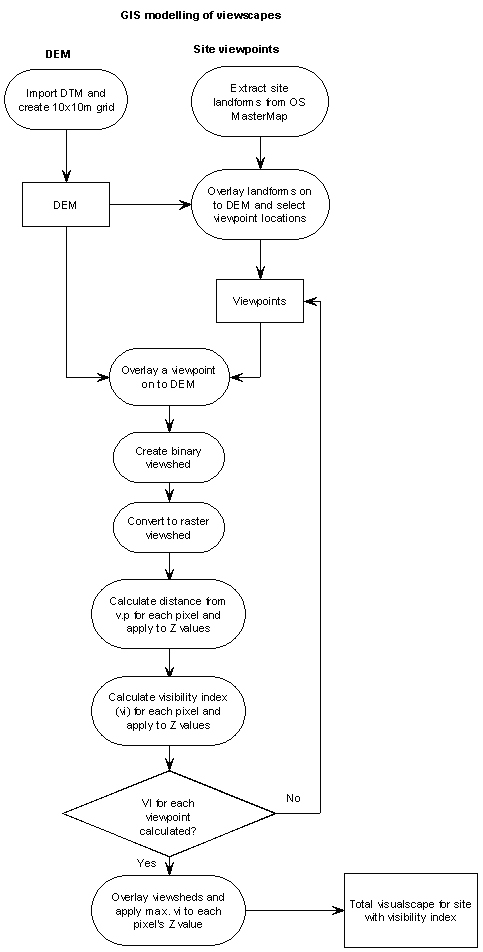
The data processing and analysis was
carried out using two GIS
programs: Manifold GIS version
8.0 and Global Mapper version 9.0 (details are listed in appendix 1).
Creating the Digital Elevation Model (DEM)
To create the DEM, Ordnance Survey 1:10 000 scale Landform Profile DTM data was downloaded from Digimap (for details about the Edina Digimap service see the appendix). The data is supplied as 5x5km tiles in NTF format and twenty tiles were required to cover the Gower study area. The data tiles were imported into Global Mapper to create a composite DEM consisting of approximately 5,775,000 10m x 10m cells. The data was imported without interpolation or generalisation so that the optimum precision was maintained.
Selecting site viewpoints
The conventional approach to viewshed calculation has been to take a single viewpoint as the observer’s position. This would suffice for a standing stone or summit location as the view would be as seen by an observer as they turned around on the same spot. The views from a hillfort however can change significantly as the observer moves around the site and so the use of multiple viewpoints is essential to build a composite viewshed which takes in the full range of views (Gillings and Wheatley, 2001, 12).
The number of viewpoints and their individual locations for each hillfort was determined by its size, aspect and structure. As a result the number of viewpoints per location ranged from four to ten. The viewpoints were selected from locations along the top of banks, both at the angles and at approximate mid-points, reflecting the variance in heights resulting from the sloping aspect of some of the sites, notably The Bulwark and Hardings Down. Initially the viewpoints were to have been selected by visiting each site and taking GPS readings, but difficulties over access and excessive vegetation growth made this approach impractical. An alternative method was therefore adopted, utilising Ordnance Survey MasterMap data. This is supplied as vector data at 1:2500 scale in multiple layers, one of which depicts landforms which include banks and ditches of the hillforts. MasterMap data for the hillfort areas was downloaded from Digimap and imported into MapInfo 8.0. The landforms for each site were extracted and imported into Global Mapper. The landform objects were then overlaid on to the DEM, which enabled the heights along and across the banks to be examined and suitable viewpoints selected. Figure 2 shows part of The Bulwark as depicted by the Landform Profile data overlaid on to MasterMap:
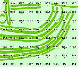
Figure 2: OS Landform Profile heights for part of The Bulwark
© Height data Crown Copyright/database right 2012 (An Ordnance Survey/EDINA supplied service)
Generating the binary viewsheds
Using the viewpoints for each site, the initial binary viewsheds could then be generated. Global Mapper allows a number of input parameters to be entered and the following were used:
Observer elevation: 1.7m
Target height: 0.5m
Radius: 4.816 km
The observer height represents the eye-level of a typical Iron Age male and the target height was set to 0.5m above ground level to avoid excessive fragmentation of the viewshed which caused by small variations in the height of pixels. The radius was set to 4.816km as this represents the distance at which the visibility index reduces to 0.1 which as explained in chapter 2 represents the extreme limit of visibility.
The results for The Bulwark are a good example of the variation in viewshed area and direction from each viewpoint and these are discussed and illustrated in the following figures. The viewpoints occupy a range of positions, encompassing the overall layout of the site. They represent the changing aspect viewed by an observer moving around both the central part of the hillfort and the outer defensive banks. The separate viewsheds are illustrated in Figure 3 and the areas covered by each viewshed are compared in figure 4.
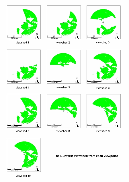
Figure 3: The Bulwark - variation in viewshed direction and area
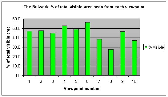
Figure 4: The Bulwark - Variation in % coverage
Figure 4 illustrates the wide variation in direction and coverage at each viewpoint. The average viewpoint coverage is 44.8% of the total area within a 4.816 km radius of the viewpoint. Interestingly even the highest viewpoint (no. 9: 173m) covers less than 50% of the total area, so taking a range of viewpoints is essential to create a realistic total viewshed.
Creating the fuzzy viewsheds
The binary viewsheds were imported into Manifold for subsequent processing, as Global Mapper does not support sophisticated raster queries and calculations. Each binary viewshed was converted to a fuzzy viewshed in two steps. First the Z value of each pixel in the viewshed was changed from the height to the distance from the viewpoint, by using a geographic update query to modify the value. The process calculates the spherical distance (allowing for the curvature of the earth) from the viewpoint’s X and Y coordinates to the centre X and Y coordinates of each pixel. Next, the formula given in chapter 2 was used to modify the Z distance value of each pixel to represent the visibility index. This was performed by a non-geographic update query (as this step is purely mathematical and does not use intrinsic spatial values) and the process repeated for each viewshed.
To create the composite
total viewshed for the area the individual viewsheds were combined using a
conditional argument which allocated the highest visibility value from each of
the overlapping viewsheds to the Z value of the composite viewshed. The composite viewshed was then overlaid on
the DEM, using graduated colours used to depict the visibility index. The colours were allocated to the visibility
index range with green representing a value of 1.0, through yellow for a value
of 0.33, to orange and finally red for the extreme limit where the value = 0.1.The
results are presented and discussed in Part Four: Results and Discussion.
Part Two: GIS surface analysis in archaeology
Part Four: Results and discussion
© Estate of Nigel James 2013