Part Four: Results and discussion
Part Two: GIS surface analysis in archaeology
Historical background
The use of visibility and inter-visibility analysis in archaeology to attempt to understand the spatial pattern of site location has a long history. This was often a textual depiction of the view towards or from a particular site (Lock, 2003, 165) and the antiquary William Stukeley noted the significance in the location of barrows to create a ‘false horizon’ (Van Leusen, 2002, 6-9). The problem with the visual approach is the human impact on the landscape since the time the monuments were constructed. A simple visual assessment of the inter-visibility between locations is now often hampered by buildings and trees, preventing long-distance viewing except in undeveloped remote locations. In the past, attempts were sometimes made to circumvent this problem by removing obstructions. Sir Norman Lockyer’s investigations into alignments centred on the Merry Maidens stone circle in Cornwall involved the removal of sections of walls (Mitchell, 1974, 63) but this is would probably be unacceptable today!
The GIS approach
The use of surface
analysis in a Geographic Information System (GIS) provides a possible
solution. The GIS approach has been
criticised in the past, in particular the geographic nature of GIS which treats
landscapes as an abstract geographic object (termed ‘Cartesian space’), without
the human and historic perspective (Van Leusen, 2002, 6-2), viewed as a revival
of environmental determinism, advocated by the processualist approach to
archaeology. The rigid nature of
analysis using GIS was considered naïve and over-simplistic, reducing the nature of
cognitive space to a binary visible/not visible area covering an infinite
distance, yet despite these criticisms the use of binary viewsheds in
archaeology has become well established. Published research appears to fall into two
broad categories. The first uses binary
viewshed analysis alone to test the possible reasons behind the location of monuments
and structures in the landscape, using inter-visibility as a determining factor. The second approach uses viewsheds in
combination with other physiographic data (such as slope and aspect of the area
within the viewshed) to establish the influence of the landscape on location,
as view alone is just one of many possible reasons for the choice of site.
An example using binary viewshed analysis for testing location is a study by Lock and Harris on the barrows of the Danebury area, cited by Wheatley (Wheatley, 1995) which suggested deliberate placement to avoid inter-visibility with other barrows. When applied to defensive structures such as hillforts, the limited overlap between viewsheds could indicate a planned distribution intended to maximise visual surveillance, by maintaining continuous observation with a minimum number of monitoring sites. It could also reflect the desire to create territories with boundaries at the limits of vision.
By combining the viewshed with other landscape data it is possible to move beyond the simple binary test of visibility to include other factors which could influence the choice of location. The Iron Age has left little evidence of farming and settlement outside the surviving forts and enclosures, but such land use could have been significant if the purpose of a hillfort was to overlook a territory. In this case the need for visibility was not just defensive but to observe and control the surrounding area and possibly act as an administrative focus and place of refuge for people and animals.
It is possible to
suggest likely areas used for agriculture by analysis of slope and aspect, both
of which can be determined from digital elevation data using a GIS. The maximum
slope which is compatible with agriculture depends on the method of working the
land, especially ploughing with animals.
It has been proposed that a slope angle of up to 25% could probably be
worked by human labour, but plough animals could not cope with this, so 13%
would be their upper limit (Van Joolen, 2003, 28). A southerly aspect would be favoured to
optimise solar exposure and this can be determined in a similar way to slope,
but using the maximum rate of change in elevation between cells (Chapman, 2006,
83).
Visibility analysis methods in GIS: Line of sight and viewsheds
Inter-visibility between two sites can be determined by the use of line of sight analysis. The method is straightforward – the terrain profile along a straight line between two points is analysed using elevation data in a GIS. Inter-visibility is true if no intermediate points are higher than either the observer’s position or the target. Figure 1 shows this is the case between The Bulwark and Cil Ifor :
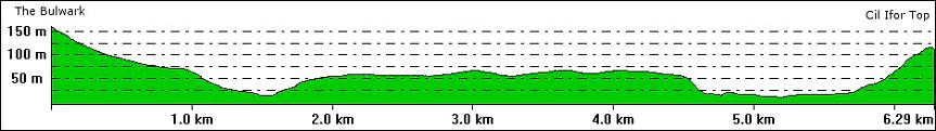
Figure 1: Line of sight profile between The Bulwark and Cil Ifor
Line of site
analysis helps to circumvent the problems noted earlier such as obstructions
resulting from later development and changes in land cover, such as planting
woodlands. Under favourable conditions the technique can be applied in field
observations, but the limiting factor is the inability to test more than one
target at a time. To explore the
positional significance of a site it is necessary to consider the entire visual
landscape surrounding the site. This can be from the point of view of observing
(looking out from the site across the landscape) which would be an important
factor for a defensive structure or sighting point used to observe solar or
other astronomical events. Conversely
the site may have been located for visual significance, in which case the area
from which the site can be observed has to be determined. This requires the use of multiple line of
sight tests to establish a viewshed, which
determines visible and non-visible areas as viewed from the observer’s position. The resulting pattern can then be
superimposed on a cartographic representation of the landscape to reveal the
visible areas.
Until the development of digital cartography and geographic analysis software (GIS) creating viewsheds was a laborious process. A viewshed examines the line of sight from an observer’s location to a number of points in the landscape and without the use of computational methods this would have to be limited to sample points, or the maual plotting of points from contours (isolines linking points of similar height).
Modelling the terrain
Most GIS programs use surface data in a raster format to analyse surfaces. A raster consists of a regular grid of cells encoded with the height of the cell, which can then be used to compute the viewshed. If the source data is at a larger resolution than that required for the surface model, or the spatial distribution is irregular, interpolation is required to estimate values for cells which do not correspond to known values. Data can be derived from contours and using a GIS it is a straightforward process to extract points at regular intervals along a contour line. If this process is repeated for all contours within a defined area a set of source data points will be produced.
An alternative
method of computing a surface from heights is the triangulated irregular
network (TIN). This uses Delaunay
Triangles (a method of triangulation using the three points which fall on the
circumference of the smallest circle which contains the points). The result is a faceted surface which has the
additional function of depicting slope and aspect (Chapman, 2006, 73). To examine the overlap between viewsheds (and
conversely to see how many sites are visible for a given location in the
landscape) the cellular structure of a raster surface is required to perform
map algebra, which is not possible using TINs. The viewsheds are combined and
the binary values summed (with 1 subtracted from each cell to allow for a site
‘seeing itself’) to create a single multiple viewshed.
Source data
The source elevation data used in this project is the Ordnance Survey Landform-Profile DTM data set. Although the Ordnance Survey refer to this as a DTM (digital terrain model), it is more accurately a DEM (digital elevation model). DTMs normally incorporate slope and aspect information (Albrecht, 2007, 62), whereas the Ordnance Survey product only has a height attribute.
The digital elevation data is in the form of a 10mx10m grid. Heights are given to 1cm but the source data (1:10,000 scale contour mapping and air survey) is not necessarily to this level of precision. The Ordnance Survey literature gives a root mean square error (the standard measure of error used in surveying) of +/- 1m (Ordnance Survey, 2001, 3.3). Ordnance Survey do not give further information as to whether the error varies by location and the single figure is effectively a nationwide calculation. The error in the height data will in turn affect the accuracy of any viewshed calculations, but this can be allowed for by calculating the probable accuracy of the result, for example by using Monte Carlo simulation. This uses a random value (in this case it would range from -1 to +1) which is added to each height value. The viewshed is then calculated using the modified values. The process will have to be repeated n times and the results averaged to obtain a probable viewshed (Kidner et. al., 2001, 27). This process would be extremely time-consuming and beyond the scope of this project. The viewsheds from the Gower forts extend many kilometres and the effect of a 1 metre error will become insignificant with distance, so the DTM data will be used unmodified. A further characteristic of the DTM data is the smoothing effect of the 10m sampling grid. A cell size less than 10m can be interpolated to create cells with intermediate values which would model slope more realistically between grid points, but ridges or dips between the 10m points will not be recorded. Whilst this would be significant in small-area surface modelling, the surface model will have the same characteristics over the entire area of Gower, so it can probably be ignored for the scale of this project. Of more significance is the assumed certainty of visual state in a binary viewshed and this is addressed in the next section.
Introducing uncertainty into viewshed calculation
Simple binary viewsheds can have one state, visible or not visible. In reality this is over simplistic as view is affected by factors such as distance and viewing conditions. This cannot be modelled in a binary viewshed as values within a range from visible (1) through decreasing degrees of clarity to invisible (0) are rquired.
The effects of human visual acuity are complex and inter-related, resulting in psychophysical limits to vision (Ogburn, 2006, 406). There are three principal measures: detection acuity (the ability to see a small target against a dark background), resolution acuity (separating the elements of target) and recognition stimulus (recognising and identifying a target). These are measured by the angle subtended by the target object as seen by the observer. In simple terms this means that for a target of given size, the observer’s ability to recognise, separate discrete parts or simply detect the object will depend on distance.
One approach to this problem is the use of Higuchi viewsheds, which replace the single viewshed with a series of zones or distance classes which reflect the observer’s ability to recognise features in the landscape (Wheatley and Gillings, 2000, 12). Higuchi used the width of a tree as the observed object and proposed eight zones which represented the progressive reduction in the observer’s acuity. For convenience these can be reduced to three, representing foreground, middle ground and distant ground. In the foreground zone the observer can see sufficient detail to recognise the tree species from shape and leaf type (recognition zone). With increasing distance this is reduced to a middle-distance view (resolution), where the number of trees can be detected but not in sufficient detail to identify the species) leading finally to a distant view (detection) where colour contrast might suggest trees but only as a contiguous group.
For an observer to be able to detect, resolve and identify a target object it has to occupy at least 1° of arc. As the arc decreases the object moves into middle zone until the arc is 3', at which point the distant zone commences. The limit of the distant zone for a person with normal vision is an arc of 1', in perfect conditions of visibility and 20/20 vision the minimum is 30" of arc, but this is the extreme limit and for an observer with average eyesight an arc of 1’ is considered the minimum (Ogburn, 2006, 410).
From these visual arcs it is possible to define distances for the three zones, using the trigonometric relationship between the visual arc, distance from observer and object width:
tan (b/2) = s/2d
(where b = visual arc; s = object width and d = distance from observer)
This can then be adapted to enable a distance multiplier a to be calculated, which multiplied by s gives the value of d for an object of given width:
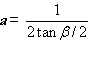
It is clear that the value of a will vary according to target width. Ogburn used a target width of 1 metre for these calculations and the results are shown in figure 2:
|
Visual arc |
Distance multiplier |
Distance (m) for object of width |
Notes |
||
|
1m |
2m |
5m |
|||
|
30" |
6880 |
6880 |
13700 |
34400 |
Limit of perfect acuity |
|
1' |
3440 |
3440 |
6880 |
17200 |
Limit of normal vision |
|
3' |
1150 |
1150 |
2300 |
5750 |
Limit of middle ground zone |
|
1° |
57 |
57 |
114 |
290 |
Limit of foreground zone |
Figure 2: Distance Multipliers for a range of visual arcs and object sizes (source: Ogburn, 2006)
Wheatley and Gillings suggest using the height of the observed object (in their case, a tree) to calculate the distance multipliers, but visual arc is a horizontal angle (human vision has greater resolving power horizontally then vertically). This inconsistency was noted by Ogburn with an example of Californian Redwood trees, which by virtue of their height would create distance zones significantly larger than in deserts for example, even though the latter would have superior visibility with their lack of obstructions and clear climate (Ogburn, 2006, 408). To avoid this confusion I propose using the width of a person (rather than the height) which will be used to modify the parameters used to generate the initial binary viewshed. Taking a value of 0.7m for this, the recalculated distances are shown in figure 3:
|
Visual arc |
Distance multiplier |
Distance (m) from observer |
Notes |
|
|
30" |
6880 |
4816 |
Limit of perfect acuity |
|
|
1' |
3440 |
2408 |
Limit of normal vision |
|
|
3' |
1150 |
805 |
Limit of middle ground zone |
|
|
1° |
57 |
39.9 |
Limit of foreground zone |
Figure 3: Modified distance table for width of one person
Although the Higuchi zonal system improves on the binary viewshed, visibility
would reduce progressively once the limit of clear observation was passed (the
transition between the foreground and middle ground zones). An infinite number of zones are required to represent
the change in visibility but in practice this problem can be addressed by introducing uncertainty (Gillings, 1998, 117). A method
of modelling this is the introduction of ‘fuzziness’ to the result (Wheatley
and Gillings, 2000, 9), by using the distance from the observer’s position as a
weighting factor to modify the visibility value. This produces a more realistic
result than the fixed Higuchi ranges.
The notion of
using fuzzy set theory to modify the viewshed was proposed by Fisher, who used
it in conjunction with distance decay (Fisher, 1994 in Wheatley and Gillings,
2000, 8). It as been noted that Fisher
initially misused the term “fuzzy viewshed”, by applying it to RSME errors in
the DEM, a problem better addressed by using Monte-Carlo Simulation. Fisher corrected this in subsequent work, but
it has still been misapplied in archaeological studies (Ogburn, 2006,
408). The Fisher model for a basic fuzzy
viewshed assumes that perfect clarity exists to the edge of the foreground zone
(viewshed value = 1) and then progressively decreases with distance up to the
edge of the middle zone, from which point visibility has little clarity and
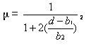
degrades further until extinction (viewshed value = 0). The formula used by Fisher was based on
earlier work on fuzzy sets and is shown below:
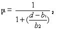
Fuzzy membership (visibility) is represented by μ, with b1 and b2 representing the limits of the foreground and middle zones respectively. Distance from the observer is represented by d. The value of μ will be 1 to the edge of the foreground zone and then decrease progressively towards 0. The value b2 will be the distance at which μ = 0.5. This defines the point at which visibility starts to fall noticeably and the observed object subtends an arc of 1'. Using the proposed value of 0.7, the progressive decrease in visibility is shown in figure 9, with the limit of perfect human acuity under clear conditions (0.1) occurring at a distance of between 7000 and 7500m.
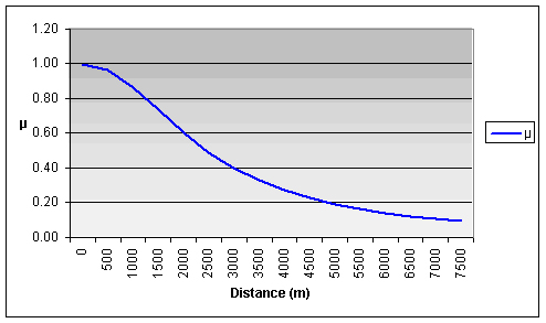
Figure 4: Decrease in visibility with distance where b2 gives a value of μ = 0.5
A problem identified by Ogburn is that the value of 0.5 is associated with a visual arc of 1', the limit beyond which a person with perfect vision can no longer identify an object. He suggests a value of nearer 0.4 which would allow for less than perfect vision and/or viewing conditions. This requires a modification of Fisher’s formula by including a multiplier (in this case 2) so a value of 0.33 for μ is achieved. This will be used for the calculations in this project.
The graph of visibility using the modified formula is shown below in figure 5:
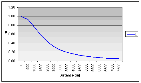
Figure 5: Decrease in visibility with distance where b2 gives a value of μ = 0.33
The use of μ = 0.33 as the value which determines the distance b2 results in a value of μ = 0.1 at the extreme limit of visibility, the point at which an object subtends 30" of arc. This is a more realistic result than using μ = 0.5 which produces a value for b2 of between 7000 and 7500, far beyond the 30" limit.
© Estate of Nigel James 2013